目标检测之边框回归入门【Tensorflow】

要学习目标检测算法吗?任何一个ML学习者都希望能够给图像中的目标物体 圈个漂亮的框框,在这篇文章中我们将学习目标检测中的一个基本概念: 边框回归/Bounding Box Regression。边框回归并不复杂,但是即使像YOLO 这样顶尖的目标检测器也使用了这一技术!

我们将使用Tensorflow的Keras API实现一个边框回归模型。现在开始吧! 如果你可以访问Google Colab的话,可以访问这里

1、准备数据集

学编程,上汇智网,在线编程环境,一对一助教指导。

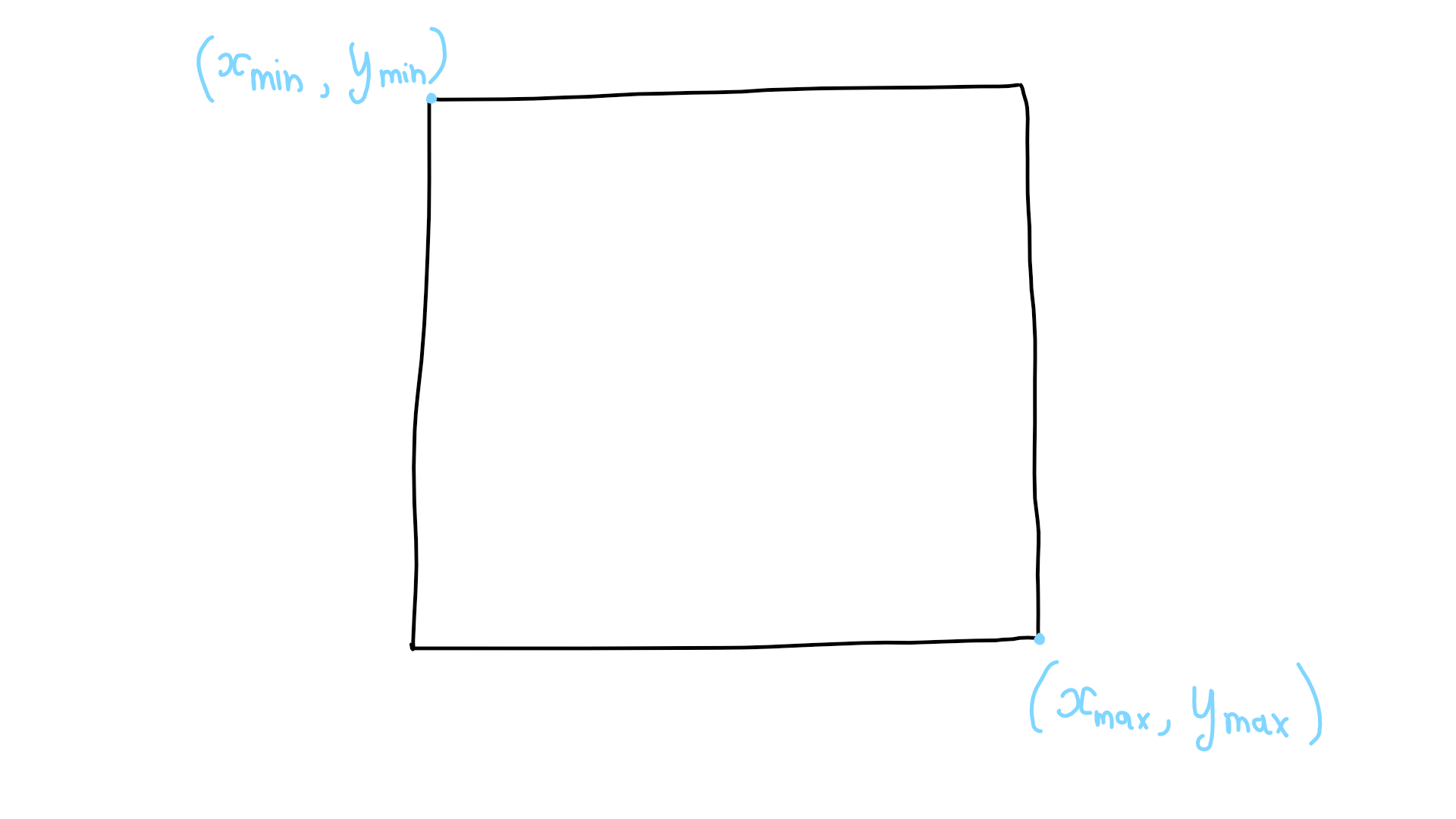
我们将使用Kaggle.com上的这个图像定位数据集, 它包含了3类(黄瓜、茄子和蘑菇)共373个已经标注了目标边框的图像文件。我们的 目标是解析图像并进行归一化处理,同时从XML格式的标注文件中解析得到目标物体 包围框的4个顶点的坐标:

如果你希望创建自己的标注数据集也没有问题!你可以使用LabelImage。 利用LabelImage你可以快速标注目标物体的包围边框,然后保存为PASCAL-VOC格式:

2、数据处理

学编程,上汇智网,在线编程环境,一对一助教指导。

首先我们需要处理一下图像。使用glob包,我们可以列出后缀为jpg的文件,逐个处理:

1
2
3
4
5
6
7
8
9
10
11
12
input_dim = 228

from PIL import Image , ImageDraw
import os
import glob

images = []
image_paths = glob.glob( 'training_images/*.jpg' )
for imagefile in image_paths:
image = Image.open( imagefile ).resize( ( input_dim , input_dim ))
image = np.asarray( image ) / 255.0
images.append( image )

接下来我们需要处理XML标注。标注文件的格式为PASCAL-VOC。我们使用xmltodict 包将XML文件转换为Python的字典对象:

1
2
3
4
5
6
7
8
9
10
11
12
13
14
15
16
17
18
import xmltodict
import os

bboxes = []
classes_raw = []
annotations_paths = glob.glob( 'training_images/*.xml' )
for xmlfile in annotations_paths:
x = xmltodict.parse( open( xmlfile , 'rb' ) )
bndbox = x[ 'annotation' ][ 'object' ][ 'bndbox' ]
bndbox = np.array([ int(bndbox[ 'xmin' ]) , int(bndbox[ 'ymin' ]) , int(bndbox[ 'xmax' ]) , int(bndbox[ 'ymax' ]) ])
bndbox2 = [ None ] * 4
bndbox2[0] = bndbox[0]
bndbox2[1] = bndbox[1]
bndbox2[2] = bndbox[2]
bndbox2[3] = bndbox[3]
bndbox2 = np.array( bndbox2 ) / input_dim
bboxes.append( bndbox2 )
classes_raw.append( x[ 'annotation' ][ 'object' ][ 'name' ] )

现在我们准备训练集和测试集:

1
2
3
4
5
6
7
8
9
10
11
from sklearn.preprocessing import LabelBinarizer
from sklearn.model_selection import train_test_split

boxes = np.array( bboxes )
encoder = LabelBinarizer()
classes_onehot = encoder.fit_transform( classes_raw )

Y = np.concatenate( [ boxes , classes_onehot ] , axis=1 )
X = np.array( images )

x_train, x_test, y_train, y_test = train_test_split( X, Y, test_size=0.1 )

3、创建Keras模型

学编程,上汇智网,在线编程环境,一对一助教指导。

我们首先为模型定义一个损失函数和一个衡量指标。损失函数同时使用 了平方差(MSE:Mean Squared Error)和交并比(IoU:Intersection over Union), 指标则用来衡量模型的准确性同时输出IoU得分:

IoU计算两个边框的交集与并集的比率:

Python实现代码如下:

1
2
3
4
5
6
7
8
9
10
11
12
13
14
15
16
17
18
19
20
21
22
23

input_shape = ( input_dim , input_dim , 3 )
dropout_rate = 0.5
alpha = 0.2

def calculate_iou( target_boxes , pred_boxes ):
xA = K.maximum( target_boxes[ ... , 0], pred_boxes[ ... , 0] )
yA = K.maximum( target_boxes[ ... , 1], pred_boxes[ ... , 1] )
xB = K.minimum( target_boxes[ ... , 2], pred_boxes[ ... , 2] )
yB = K.minimum( target_boxes[ ... , 3], pred_boxes[ ... , 3] )
interArea = K.maximum( 0.0 , xB - xA ) * K.maximum( 0.0 , yB - yA )
boxAArea = (target_boxes[ ... , 2] - target_boxes[ ... , 0]) * (target_boxes[ ... , 3] - target_boxes[ ... , 1])
boxBArea = (pred_boxes[ ... , 2] - pred_boxes[ ... , 0]) * (pred_boxes[ ... , 3] - pred_boxes[ ... , 1])
iou = interArea / ( boxAArea + boxBArea - interArea )
return iou

def custom_loss( y_true , y_pred ):
mse = tf.losses.mean_squared_error( y_true , y_pred )
iou = calculate_iou( y_true , y_pred )
return mse + ( 1 - iou )

def iou_metric( y_true , y_pred ):
return calculate_iou( y_true , y_pred )

接下来我们创建CNN模型。我们堆叠几个Conv2D层并拉平其输出, 然后送入后边的全连接层。为了避免过拟合,我们在全连接层使用Dropout, 并使用LeakyReLU激活层:

1
2
3
4
5
6
7
8
9
10
11
12
13
14
15
16
17
18
19
20
21
22
23
24
25
26
27
28
29
30
31
32
33
34
35
36
37
38
39
40
41
42
43
44
45
46
47
48
49
50
51
52
53
54
55
56
57
num_classes = 3
pred_vector_length = 4 + num_classes

model_layers = [
keras.layers.Conv2D(16, kernel_size=(3, 3), strides=1, input_shape=input_shape),
keras.layers.LeakyReLU( alpha=alpha ) ,
keras.layers.Conv2D(16, kernel_size=(3, 3), strides=1 ),
keras.layers.LeakyReLU( alpha=alpha ) ,
keras.layers.MaxPooling2D( pool_size=( 2 , 2 ) ),

keras.layers.Conv2D(32, kernel_size=(3, 3), strides=1),
keras.layers.LeakyReLU( alpha=alpha ) ,
keras.layers.Conv2D(32, kernel_size=(3, 3), strides=1),
keras.layers.LeakyReLU( alpha=alpha ) ,
keras.layers.MaxPooling2D( pool_size=( 2 , 2 ) ),

keras.layers.Conv2D(64, kernel_size=(3, 3), strides=1),
keras.layers.LeakyReLU( alpha=alpha ) ,
keras.layers.Conv2D(64, kernel_size=(3, 3), strides=1),
keras.layers.LeakyReLU( alpha=alpha ) ,
keras.layers.MaxPooling2D( pool_size=( 2 , 2 ) ),

keras.layers.Conv2D(128, kernel_size=(3, 3), strides=1),
keras.layers.LeakyReLU( alpha=alpha ) ,
keras.layers.Conv2D(128, kernel_size=(3, 3), strides=1),
keras.layers.LeakyReLU( alpha=alpha ) ,
keras.layers.MaxPooling2D( pool_size=( 2 , 2 ) ),

keras.layers.Conv2D(256, kernel_size=(3, 3), strides=1),
keras.layers.LeakyReLU( alpha=alpha ) ,
keras.layers.Conv2D(256, kernel_size=(3, 3), strides=1),
keras.layers.LeakyReLU( alpha=alpha ) ,
keras.layers.MaxPooling2D( pool_size=( 2 , 2 ) ),

keras.layers.Flatten() ,

keras.layers.Dense( 1240 ) ,
keras.layers.LeakyReLU( alpha=alpha ) ,
keras.layers.Dense( 640 ) ,
keras.layers.LeakyReLU( alpha=alpha ) ,
keras.layers.Dense( 480 ) ,
keras.layers.LeakyReLU( alpha=alpha ) ,
keras.layers.Dense( 120 ) ,
keras.layers.LeakyReLU( alpha=alpha ) ,
keras.layers.Dense( 62 ) ,
keras.layers.LeakyReLU( alpha=alpha ) ,

keras.layers.Dense( pred_vector_length ),
keras.layers.LeakyReLU( alpha=alpha ) ,
]

model = keras.Sequential( model_layers )
model.compile(
optimizer=keras.optimizers.Adam( lr=0.0001 ),
loss=custom_loss,
metrics=[ iou_metric ]
)

4、训练模型

现在可以开始训练了:

1
2
3
4
5
6
7
model.fit( 
x_train ,
y_train ,
validation_data=( x_test , y_test ),
epochs=100 ,
batch_size=3
)model.save( 'model.h5')

5、在图像上绘制边框

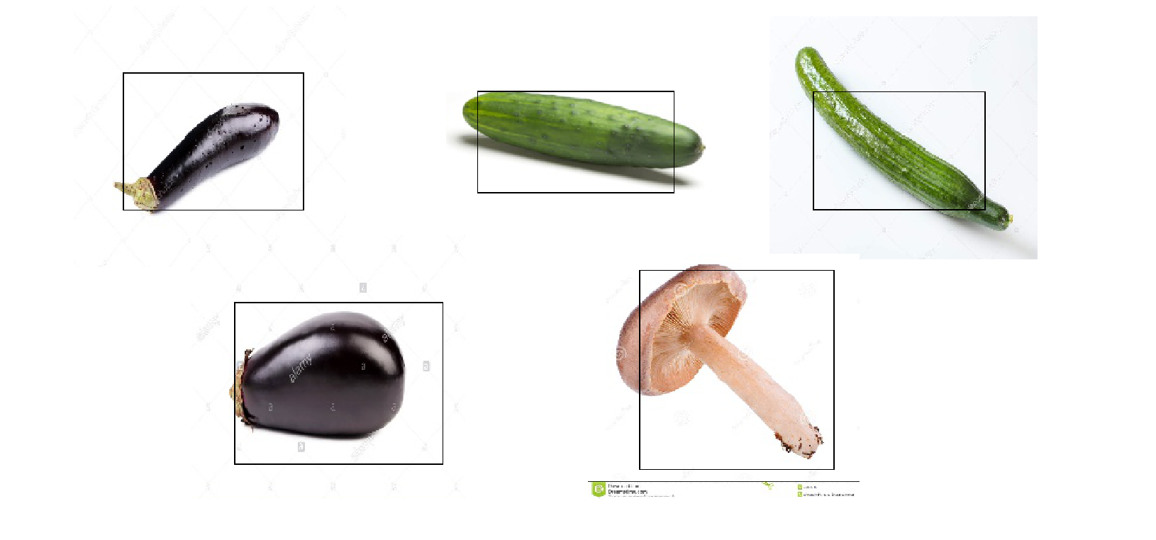
现在我们的模型已经训练好了,可以用它来检测一些测试图像 并绘制检测出的对象的边框,然后把结果图像保存下来。

1
2
3
4
5
6
7
8
9
10
!mkdir -v inference_images

boxes = model.predict( x_test )
for i in range( boxes.shape[0] ):
b = boxes[ i , 0 : 4 ] * input_dim
img = x_test[i] * 255
source_img = Image.fromarray( img.astype( np.uint8 ) , 'RGB' )
draw = ImageDraw.Draw( source_img )
draw.rectangle( b , outline="black" )
source_img.save( 'inference_images/image_{}.png'.format( i + 1 ) , 'png' )

下面是检测结果图示例:

要决定测试集上的IOU得分,同时计算分类准确率,我们使用如下的代码:

calculate_avg_iou( target_boxes , pred_boxes ):
1
2
3
4
5
6
7
8
9
10
11
12
13
14
15
16
17
18
19
20
21
22
23
24
    xA = np.maximum( target_boxes[ ... , 0], pred_boxes[ ... , 0] )
yA = np.maximum( target_boxes[ ... , 1], pred_boxes[ ... , 1] )
xB = np.minimum( target_boxes[ ... , 2], pred_boxes[ ... , 2] )
yB = np.minimum( target_boxes[ ... , 3], pred_boxes[ ... , 3] )
interArea = np.maximum(0.0, xB - xA ) * np.maximum(0.0, yB - yA )
boxAArea = (target_boxes[ ... , 2] - target_boxes[ ... , 0]) * (target_boxes[ ... , 3] - target_boxes[ ... , 1])
boxBArea = (pred_boxes[ ... , 2] - pred_boxes[ ... , 0]) * (pred_boxes[ ... , 3] - pred_boxes[ ... , 1])
iou = interArea / ( boxAArea + boxBArea - interArea )
return iou

def class_accuracy( target_classes , pred_classes ):
target_classes = np.argmax( target_classes , axis=1 )
pred_classes = np.argmax( pred_classes , axis=1 )
return ( target_classes == pred_classes ).mean()

target_boxes = y_test * input_dim
pred = model.predict( x_test )
pred_boxes = pred[ ... , 0 : 4 ] * input_dim
pred_classes = pred[ ... , 4 : ]

iou_scores = calculate_avg_iou( target_boxes , pred_boxes )
print( 'Mean IOU score {}'.format( iou_scores.mean() ) )

print( 'Class Accuracy is {} %'.format( class_accuracy( y_test[ ... , 4 : ] , pred_classes ) * 100 ))

原文链接:Getting Started With Bounding Box Regression In TensorFlow

汇智网翻译整理,转载请标明出处